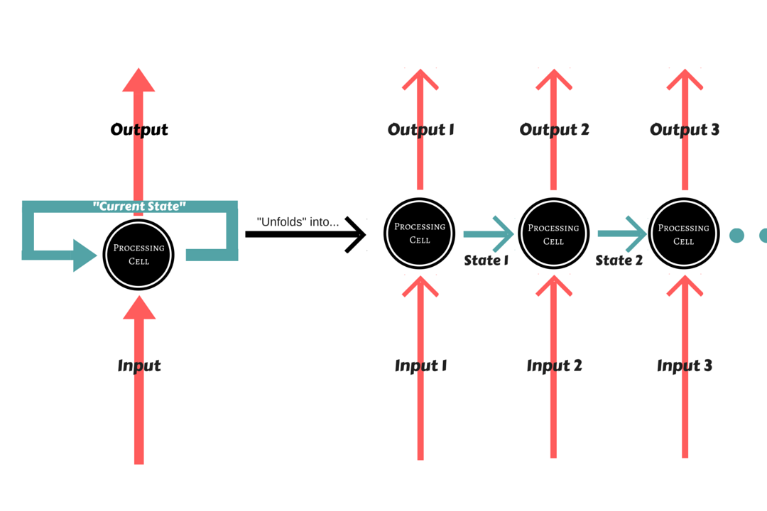
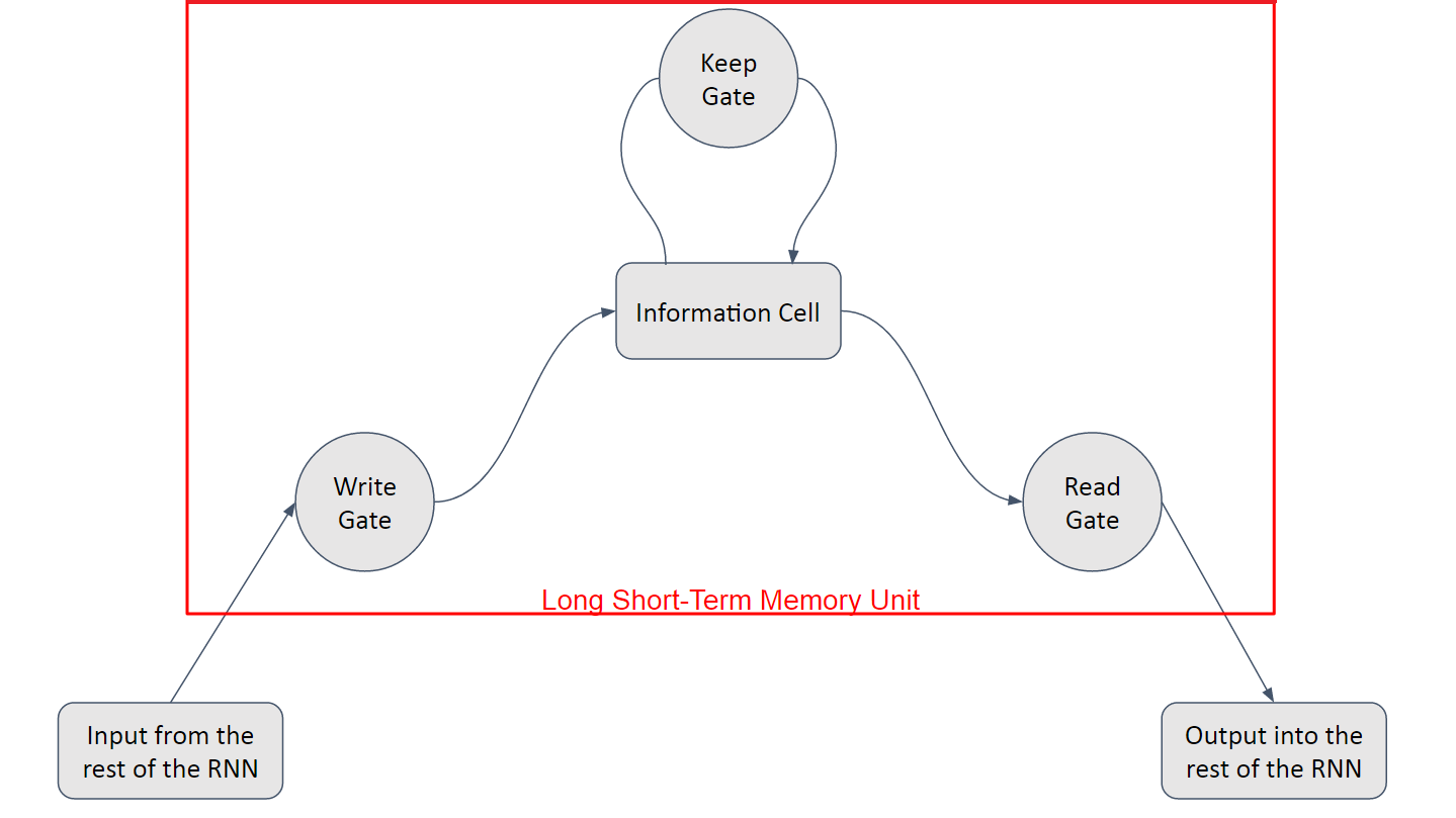
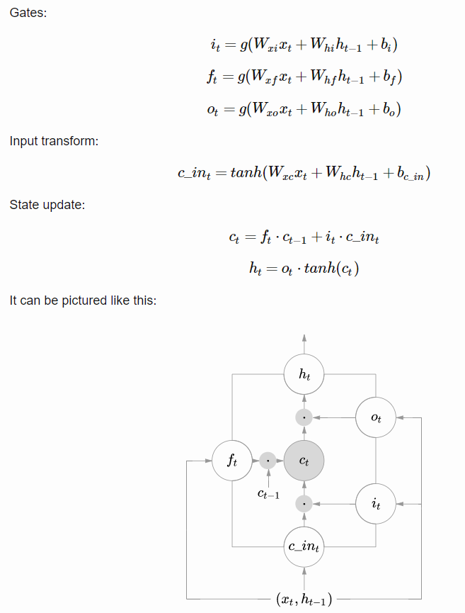
Long Short-Term Memory It is an abstraction of how computer memory works. It is “bundled” with whatever processing unit is implemented in the Recurrent Network, although outside of its flow, and is responsible for keeping, reading, and outputting information for the model. The way it works is simple: you have a linear unit, which is the information cell itself, surrounded by three logistic gates responsible for maintaining the data. One gate is for inputting data into the information cell, one is for outputting data from the input cell, and the last one is to keep or forget data depending on the needs of the network.
Thanks to that, it not only solves the problem of keeping states, because the network can choose to forget data whenever information is not needed, it also solves the gradient problems, since the Logistic Gates have a very nice derivative.
 Long Short-Term Memory Architecture
As seen before, the Long Short-Term Memory is composed of a linear unit surrounded by three logistic gates. The name for these gates vary from place to place, but the most usual names for them are:
- the “Input” or “Write” Gate, which handles the writing of data into the information cell,
- the “Output” or “Read” Gate, which handles the sending of data back onto the Recurrent Network, and
- the “Keep” or “Forget” Gate, which handles the maintaining and modification of the data stored in the information cell.

Building a LSTM with TensorFlow Although RNN is mostly used to model sequences and predict sequential data, we can still classify images using a LSTM network. If we consider every image row as a sequence of pixels, we can feed a LSTM network for classification. Lets use the famous MNIST dataset here. Because MNIST image shape is 28*28px, we will then handle 28 sequences of 28 steps for every sample.
1
2
3
4
5
6
7
8
9
10
11
12
# Importing Libraries
%matplotlib inline
import warnings
warnings.filterwarnings('ignore')

import numpy as np
import matplotlib.pyplot as plt
import tensorflow as tf

# Importing dataset
from tensorflow.examples.tutorials.mnist import input_data
mnist = input_data.read_data_sets(".", one_hot=True)
1
2
3
4
5
6
7
8
9
10
11
12
13
14
# Defining variables for train & test data
trainings = mnist.train.images
trainlabels = mnist.train.labels
testings = mnist.test.images
testlabels = mnist.test.labels

ntrain = trainings.shape[0]
ntest = testings.shape[0]
dim = trainings.shape[1]
nclasses = trainlabels.shape[1]
print ("Train Images: ", trainings.shape)
print ("Train Labels  ", trainlabels.shape)
print ("Test Images:  " , testings.shape)
print ("Test Labels:  ", testlabels.shape)
Train Images:  (55000, 784)
Train Labels   (55000, 10)
Test Images:   (10000, 784)
Test Labels:   (10000, 10)
1
2
3
4
5
6
7
8
9
10
11
12
13
14
15
16
17
18
19
20
# Defining Network Parameters
sess = tf.InteractiveSession()

n_input = 28 # MNIST data input (img shape: 28*28)
n_steps = 28 # timesteps
n_hidden = 128 # hidden layer num of features
n_classes = 10 # MNIST total classes (0-9 digits)

learning_rate = 0.001
training_iters = 100000
batch_size = 100
display_step = 10

# The input should be a Tensor of shape: [batch_size, time_steps, input_dimension], but in our case it would be (?, 28, 28)
x = tf.placeholder(dtype="float", shape=[None, n_steps, n_input], name="x") # Current data input shape: (batch_size, n_steps, n_input) [100x28x28]
y = tf.placeholder(dtype="float", shape=[None, n_classes], name="y")

# Randoming initializing weights & biases
weights = { 'out': tf.Variable(tf.random_normal([n_hidden, n_classes])) }
biases = {'out': tf.Variable(tf.random_normal([n_classes])) }
{'out': <tf.Variable 'Variable_8:0' shape=(128, 10) dtype=float32_ref>}
Let’s Understand the parameters, inputs and outputs \({\Delta{S}}= S({\mu \Delta{t}}+{\sigma \epsilon \sqrt{\Delta{t}}})\) We will treat the MNIST image \(\in \mathcal{R}^{28 \times 28}\) as \(28\) sequences of a vector \(\mathbf{x} \in \mathcal{R}^{28}\).
Our simple RNN consists of
- One input layer which converts a $28*28$ dimensional input to an $128$ dimensional hidden layer,
- One intermediate recurrent neural network (LSTM)
- One output layer which converts an $128$ dimensional output of the LSTM to $10$ dimensional output indicating a class label.
1
2
3
#Lets design our LSTM Model
#Lets define a lstm cell with tensorflow
lstm_cell = tf.contrib.rnn.BasicLSTMCell(n_hidden, forget_bias=1.0)

1
2
3
#__dynamic_rnn__ creates a recurrent neural network specified from __lstm_cell__:
outputs, states = tf.nn.dynamic_rnn(lstm_cell, inputs=x, dtype=tf.float32)
print(outputs)
Tensor("rnn_3/transpose:0", shape=(?, 28, 128), dtype=float32)
The output of the rnn would be a [100x28x128] matrix. we use the linear activation to map it to a [?x10 matrix]
1
2
3
output = tf.reshape(tf.split(outputs, 28, axis=1, num=None, name='split')[-1],[-1,128])
print(output)
pred = tf.matmul(output, weights['out']) + biases['out']
Tensor("Reshape_1:0", shape=(?, 128), dtype=float32)
1
2
3
#Now, we define the cost function and optimizer:
cost = tf.reduce_mean(tf.nn.softmax_cross_entropy_with_logits(labels=y, logits=pred ))
optimizer = tf.train.AdamOptimizer(learning_rate=learning_rate).minimize(cost)
1
2
3
#Here we define the accuracy and evaluation methods to be used in the learning process:
correct_pred = tf.equal(tf.argmax(pred,1), tf.argmax(y,1))
accuracy = tf.reduce_mean(tf.cast(correct_pred, tf.float32))
1
2
3
4
5
6
7
8
9
10
11
12
13
14
15
16
17
18
19
20
21
22
23
24
25
26
27
28
29
30
31
32
33
34
35
36
#Running the tensorflow graph

init = tf.global_variables_initializer()
with tf.Session() as sess:
    sess.run(init)
    step = 1
    #Keep training until reach max iterations
    while step * batch_size < training_iters:
        #We will read a batch of 100 images [100 x 784] as batch_x
        #batch_y is a matrix of [100x10]
        batch_x, batch_y = mnist.train.next_batch(batch_size)

        #We consider each row of the image as one sequence
        #Reshape data to get 28 seq of 28 elements, so that, batxh_x is [100x28x28]
        batch_x = batch_x.reshape((batch_size, n_steps, n_input))

        #Run optimization op (backprop)
        sess.run(optimizer, feed_dict={x: batch_x, y: batch_y})

        if step % display_step == 0:
            #Calculate batch accuracy
            acc = sess.run(accuracy, feed_dict={x: batch_x, y: batch_y})
            #Calculate batch loss
            loss = sess.run(cost, feed_dict={x: batch_x, y: batch_y})
            print("Iter " + str(step*batch_size) + ", Minibatch Loss= " + \
                  "{:.6f}".format(loss) + ", Training Accuracy= " + \
                  "{:.5f}".format(acc))
        step += 1
    print("Optimization Finished!")

    #Calculate accuracy for 128 mnist test images
    test_len = 128
    test_data = mnist.test.images[:test_len].reshape((-1, n_steps, n_input))
    test_label = mnist.test.labels[:test_len]
    print("Testing Accuracy:", \
        sess.run(accuracy, feed_dict={x: test_data, y: test_label}))
Iter 1000, Minibatch Loss= 1.933472, Training Accuracy= 0.37000
Iter 2000, Minibatch Loss= 1.606309, Training Accuracy= 0.43000
Iter 3000, Minibatch Loss= 0.963089, Training Accuracy= 0.71000
Iter 4000, Minibatch Loss= 1.097585, Training Accuracy= 0.62000
Iter 5000, Minibatch Loss= 0.703452, Training Accuracy= 0.83000
Iter 6000, Minibatch Loss= 0.712294, Training Accuracy= 0.76000
Iter 7000, Minibatch Loss= 0.670404, Training Accuracy= 0.81000
Iter 8000, Minibatch Loss= 0.693029, Training Accuracy= 0.79000
Iter 9000, Minibatch Loss= 0.555051, Training Accuracy= 0.84000
Iter 10000, Minibatch Loss= 0.482296, Training Accuracy= 0.83000
Iter 11000, Minibatch Loss= 0.350409, Training Accuracy= 0.89000
Iter 12000, Minibatch Loss= 0.500721, Training Accuracy= 0.85000
Iter 13000, Minibatch Loss= 0.434465, Training Accuracy= 0.87000
Iter 14000, Minibatch Loss= 0.472183, Training Accuracy= 0.85000
Iter 15000, Minibatch Loss= 0.361986, Training Accuracy= 0.92000
Iter 16000, Minibatch Loss= 0.363566, Training Accuracy= 0.87000
Iter 17000, Minibatch Loss= 0.427272, Training Accuracy= 0.88000
Iter 18000, Minibatch Loss= 0.164176, Training Accuracy= 0.93000
Iter 19000, Minibatch Loss= 0.245829, Training Accuracy= 0.93000
Iter 20000, Minibatch Loss= 0.424129, Training Accuracy= 0.89000
Iter 21000, Minibatch Loss= 0.302764, Training Accuracy= 0.92000
Iter 22000, Minibatch Loss= 0.175201, Training Accuracy= 0.95000
Iter 23000, Minibatch Loss= 0.152372, Training Accuracy= 0.95000
Iter 24000, Minibatch Loss= 0.251987, Training Accuracy= 0.93000
Iter 25000, Minibatch Loss= 0.297091, Training Accuracy= 0.91000
Iter 26000, Minibatch Loss= 0.183512, Training Accuracy= 0.94000
Iter 27000, Minibatch Loss= 0.219182, Training Accuracy= 0.93000
Iter 28000, Minibatch Loss= 0.184373, Training Accuracy= 0.95000
Iter 29000, Minibatch Loss= 0.286563, Training Accuracy= 0.91000
Iter 30000, Minibatch Loss= 0.185106, Training Accuracy= 0.95000
Iter 31000, Minibatch Loss= 0.275044, Training Accuracy= 0.91000
Iter 32000, Minibatch Loss= 0.185621, Training Accuracy= 0.94000
Iter 33000, Minibatch Loss= 0.188341, Training Accuracy= 0.96000
Iter 34000, Minibatch Loss= 0.281465, Training Accuracy= 0.91000
Iter 35000, Minibatch Loss= 0.170878, Training Accuracy= 0.94000
Iter 36000, Minibatch Loss= 0.223444, Training Accuracy= 0.96000
Iter 37000, Minibatch Loss= 0.200424, Training Accuracy= 0.93000
Iter 38000, Minibatch Loss= 0.175202, Training Accuracy= 0.93000
Iter 39000, Minibatch Loss= 0.136904, Training Accuracy= 0.95000
Iter 40000, Minibatch Loss= 0.139381, Training Accuracy= 0.95000
Iter 41000, Minibatch Loss= 0.175901, Training Accuracy= 0.95000
Iter 42000, Minibatch Loss= 0.237920, Training Accuracy= 0.92000
Iter 43000, Minibatch Loss= 0.115571, Training Accuracy= 0.97000
Iter 44000, Minibatch Loss= 0.119071, Training Accuracy= 0.97000
Iter 45000, Minibatch Loss= 0.122970, Training Accuracy= 0.95000
Iter 46000, Minibatch Loss= 0.167040, Training Accuracy= 0.95000
Iter 47000, Minibatch Loss= 0.211665, Training Accuracy= 0.92000
Iter 48000, Minibatch Loss= 0.122999, Training Accuracy= 0.98000
Iter 49000, Minibatch Loss= 0.136998, Training Accuracy= 0.96000
Iter 50000, Minibatch Loss= 0.147630, Training Accuracy= 0.93000
Iter 51000, Minibatch Loss= 0.137437, Training Accuracy= 0.96000
Iter 52000, Minibatch Loss= 0.169895, Training Accuracy= 0.96000
Iter 53000, Minibatch Loss= 0.178102, Training Accuracy= 0.94000
Iter 54000, Minibatch Loss= 0.117220, Training Accuracy= 0.96000
Iter 55000, Minibatch Loss= 0.120901, Training Accuracy= 0.95000
Iter 56000, Minibatch Loss= 0.148943, Training Accuracy= 0.94000
Iter 57000, Minibatch Loss= 0.151606, Training Accuracy= 0.95000
Iter 58000, Minibatch Loss= 0.134420, Training Accuracy= 0.97000
Iter 59000, Minibatch Loss= 0.191544, Training Accuracy= 0.97000
Iter 60000, Minibatch Loss= 0.150019, Training Accuracy= 0.94000
Iter 61000, Minibatch Loss= 0.117968, Training Accuracy= 0.95000
Iter 62000, Minibatch Loss= 0.039715, Training Accuracy= 0.99000
Iter 63000, Minibatch Loss= 0.153013, Training Accuracy= 0.97000
Iter 64000, Minibatch Loss= 0.110695, Training Accuracy= 0.97000
Iter 65000, Minibatch Loss= 0.095258, Training Accuracy= 0.98000
Iter 66000, Minibatch Loss= 0.072665, Training Accuracy= 0.98000
Iter 67000, Minibatch Loss= 0.091820, Training Accuracy= 0.97000
Iter 68000, Minibatch Loss= 0.120889, Training Accuracy= 0.95000
Iter 69000, Minibatch Loss= 0.061326, Training Accuracy= 0.97000
Iter 70000, Minibatch Loss= 0.075946, Training Accuracy= 0.98000
Iter 71000, Minibatch Loss= 0.117051, Training Accuracy= 0.94000
Iter 72000, Minibatch Loss= 0.087310, Training Accuracy= 0.98000
Iter 73000, Minibatch Loss= 0.228232, Training Accuracy= 0.94000
Iter 74000, Minibatch Loss= 0.027068, Training Accuracy= 0.99000
Iter 75000, Minibatch Loss= 0.129673, Training Accuracy= 0.97000
Iter 76000, Minibatch Loss= 0.073615, Training Accuracy= 0.97000
Iter 77000, Minibatch Loss= 0.104501, Training Accuracy= 0.97000
Iter 78000, Minibatch Loss= 0.100274, Training Accuracy= 0.97000
Iter 79000, Minibatch Loss= 0.097675, Training Accuracy= 0.97000
Iter 80000, Minibatch Loss= 0.093080, Training Accuracy= 0.99000
Iter 81000, Minibatch Loss= 0.129266, Training Accuracy= 0.96000
Iter 82000, Minibatch Loss= 0.018254, Training Accuracy= 1.00000
Iter 83000, Minibatch Loss= 0.041858, Training Accuracy= 0.98000
Iter 84000, Minibatch Loss= 0.056465, Training Accuracy= 0.99000
Iter 85000, Minibatch Loss= 0.078310, Training Accuracy= 0.97000
Iter 86000, Minibatch Loss= 0.078025, Training Accuracy= 0.98000
Iter 87000, Minibatch Loss= 0.059286, Training Accuracy= 0.98000
Iter 88000, Minibatch Loss= 0.044994, Training Accuracy= 0.98000
Iter 89000, Minibatch Loss= 0.067469, Training Accuracy= 0.97000
Iter 90000, Minibatch Loss= 0.120520, Training Accuracy= 0.97000
Iter 91000, Minibatch Loss= 0.134578, Training Accuracy= 0.95000
Iter 92000, Minibatch Loss= 0.108894, Training Accuracy= 0.98000
Iter 93000, Minibatch Loss= 0.195460, Training Accuracy= 0.95000
Iter 94000, Minibatch Loss= 0.136422, Training Accuracy= 0.96000
Iter 95000, Minibatch Loss= 0.133352, Training Accuracy= 0.95000
Iter 96000, Minibatch Loss= 0.153451, Training Accuracy= 0.96000
Iter 97000, Minibatch Loss= 0.087002, Training Accuracy= 0.96000
Iter 98000, Minibatch Loss= 0.126277, Training Accuracy= 0.97000
Iter 99000, Minibatch Loss= 0.110612, Training Accuracy= 0.98000
Optimization Finished!
Testing Accuracy: 0.984375
This is the end of the Recurrent Neural Networks with TensorFlow learning notebook. There are multiple application of RNN in Language Modeling and Generating Text, Machine Translation, Speech Recognition, Generating Image Descriptions, etc. Hopefully you now have a better understanding of Recurrent Neural Networks and how to implement one utilizing TensorFlow. Thank you for reading this notebook and in the next blog I shall share image classification using CNN and we will use tensorboard to visualize how to tune the hyperparameters of the network.