Monte Carlo Method is a computational mathematical technique that allows us to interpret all probable outcomes of our decisions allowing better decision making strategies under uncertainty. The essential idea behind this method is using randomness to solve problems that might be deterministic in principle.
During a Monte Carlo simulation, values are sampled at random from the input probability distributions. Each set of samples is called an iteration, and the resulting outcome from that sample is recorded. Monte Carlo simulation does these hundreds or thousands of times, and the result is a probability distribution of possible outcomes. In this way, Monte Carlo simulation provides a much more comprehensive view of what may happen. It tells you not only what could happen, but how likely it is to happen. The larger the sample size, the more accurate the estimation of the output distributions.
Monte Carlo method in Data analysis:
-
Sampling: Here the objective is to gather information about a random object by observing many realizations of it. An example is simulation modeling, where a random process mimics the behavior of some real-life system, such as a production line or telecommunications network. Another example is found in Bayesian statistics, where Markov chain Monte Carlo (MCMC) is often used to sample from a posterior distribution.
-
Estimation: In this case, the emphasis is on estimating certain numerical quantities related to a simulation model. An example in the natural setting of Monte Carlo techniques is the estimation of the expected throughput in a production line. An example in the artificial context is the evaluation of multi-dimensional integrals via Monte Carlo techniques by writing the integral as the expectation of a random variable.
-
Optimization. The Monte Carlo Method is a powerful tool for the optimization of complicated objective functions. In many applications, these functions are deterministic and randomness is introduced artificially in order to more efficiently search the domain of the objective function. Monte Carlo techniques are also used to optimize noisy functions, where the function itself is random — for example, the result of a Monte Carlo simulation.
Advantages of Monte Carlo Simulation: Monte Carlo simulation provides a number of advantages over deterministic, or “single-point estimate” analysis:
-
Probabilistic Results: Results show not only what could happen, but how likely each outcome is.
-
Graphical Results: Because of the data Monte Carlo simulation generates, it’s easy to create graphs of different outcomes and their chances of occurrence. This is important for communicating findings to other stakeholders.
-
Correlation of Inputs: In Monte Carlo simulation, it’s possible to model interdependent relationships between input variables. It’s important for accuracy to represent how, in reality, when some factors go up, others go up or down accordingly.
-
Sensitivity Analysis: With just a few cases, deterministic analysis makes it difficult to see which variables impact the outcome the most. In Monte Carlo simulation, it’s easy to see which inputs had the biggest effect on bottom-line results.
-
Scenario Analysis: In deterministic models, it’s very difficult to model different combinations of values for different inputs to see the effects of truly different scenarios. Using Monte Carlo simulation, analysts can see exactly which inputs had which values together when certain outcomes occurred. This is invaluable for pursuing further analysis.
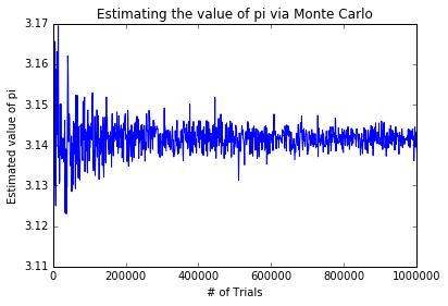
Real time application of Monte Carlo method: Determining the value of pi
#importing required packages
from random import random
import numpy as np
import matplotlib.pyplot as plt
%matplotlib inline

#Initializing variables
trials = list(np.linspace(10,1000000, 1000))
pi = []

def mc_multiple_runs(trials, hits = 0):
    for i in range(int(trials)):
        x, y = random() , random()  # generate random x,y in (0,1) at each run

        if x**2 + y**2 < 1 :  # defines the edge of the quadrant
            hits = hits + 1
    return float(hits)

for i in trials:
    pi.append(4*(mc_multiple_runs(i)/i))
# plot graphs for the value of pi determined at each trial.
plt.figure()
plt.plot(trials, pi, '-')
plt.title('Estimating the value of pi via Monte Carlo')
plt.xlabel('# of Trials')
plt.ylabel('Estimated value of pi')
plt.ylim(3.11,3.17)
plt.show()

plt.hist(pi, bins = np.linspace(3.12,3.16,50), color='green')
plt.title('Estimating the value of pi via Monte Carlo')
plt.xlabel('Estimated value of pi')
plt.ylabel('Trials')
plt.xlim(3.13,3.15)
plt.show()
In the next post, we will see the implementation of this method for determining the value at risk for stock market portfolio.
References and further reading:
- Gábor Belvárdi, “Monte Carlo simulation based performance analysis of Supply Chains“, (IJMVSC) Vol. 3, No. 2
- Dirk P. Kroese, “Why the Monte Carlo Method is so important today“, The University of Queensland
- Mike Giles, “Research on Monte Carlo Methods“, Mathematical and Computational Finance Group, Nomura, Tokyo
- “Palisade Monte Carlo simulation“, Monte Carlo Simulation
- Pamela Paxton, Patrick J. Curran, Kenneth A. Bollen, Jim Kirby, Feinian Chen, “Monte Carlo Experiments: Design and Implementation“, 288-312 Paxton Et Al.
- Book: R. Y. Rubinstein, “Simulation and the Monte Carlo Method”, John Wiley and Sons, New York (1981).